Inference Internals

Introduction

Training gets the headlines. Inference pays the bills. Every chat message, every autocomplete, every agent step is a forward pass through billions of parameters — and the engineering that makes those passes fast and cheap is some of the most interesting systems work happening today.

This guide walks through that machinery from the bottom up. We’ll start with a single token, follow it through the model, and then zoom out to see how a server juggles thousands of requests at once. Along the way you’ll find interactive figures, animations and links to the papers that introduced each idea.

Who this is for

Engineers who use language models through an API and want to understand what they are paying for. You don’t need a machine learning background — if you can read a bit of Python and know roughly what a matrix multiply is, you have everything you need.

The life of a token

A model never sees your text. It sees a sequence of integers produced by a tokenizer, which splits text into frequently occurring chunks. “Inference” becomes something like ["In", "ference"], and each chunk maps to an ID in a vocabulary of roughly 100,000 entries.

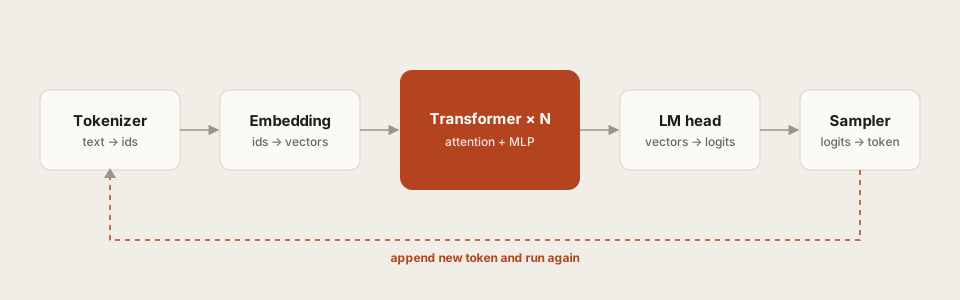
Those IDs are looked up in an embedding table, passed through a stack of transformer layers, and projected back onto the vocabulary as a vector of scores called logits. A sampler turns logits into a single choice. Then the whole thing runs again, with that new token appended.

def generate(model, prompt_ids, max_new_tokens):
    ids = prompt_ids
    for _ in range(max_new_tokens):
        logits = model(ids)[-1]          # scores for the next token
        next_id = sample(logits, temperature=0.7)
        ids = ids + [next_id]
        if next_id == EOS:
            break
    return ids

Notice the problem: this naïve loop re-processes the entire sequence on every step. Generating 1,000 tokens means 1,000 full passes over an ever-growing input. Almost every optimization in this guide is a way of not doing that.

Prefill and decode

Inference has two phases with very different personalities.

• Prefill processes the whole prompt at once. All tokens are known up front, so the work is one big parallel matrix multiply. It is compute-bound: the GPU’s arithmetic units are the bottleneck.
• Decode produces one token at a time. Each step does very little math but must read every model weight from memory. It is memory-bandwidth-bound.

Prefill is a sprint, decode is a marathon run one step at a time — and you have to reload the whole map before every step.

This split explains two numbers you see on every inference dashboard: TTFT, dominated by prefill, and inter-token latency, dominated by decode.

Arithmetic intensity

A useful back-of-envelope: a 70B-parameter model in 16-bit precision is about 140 GB of weights. A GPU with 3 TB/s of memory bandwidth needs at least $140\,\text{GB} / 3\,\text{TB/s} \approx 47\,\text{ms}$ just to stream those weights once. That is a hard floor on per-token latency for a single request — no matter how many FLOPs the chip advertises.

The KV cache

Attention lets each token look back at every token before it. To do that it computes a key and a value vector for every position in every layer. Those vectors never change once computed — so we store them. That store is the KV cache, and it turns each decode step from “reprocess everything” into “process one new token and read the cache.”

Inside each layer, a new token’s query $q_t$ is compared against every cached key $k_i$, and the scores weight the cached values $v_i$:

$$\operatorname{Attention}(q_t, K, V) = \sum_{i \le t} \operatorname{softmax}\!\left(\frac{q_t \cdot k_i}{\sqrt{d_k}}\right) v_i$$

The cache is not free. Its size grows linearly with sequence length $L$:

$$\text{KV bytes} = 2 \times n_\text{layers} \times n_\text{kv heads} \times d_\text{head} \times L \times b$$

where $b$ is the bytes per value — 2 for 16-bit precision.

For a large model with long contexts, the cache can exceed the size of the weights themselves. Managing that memory — allocating it, sharing it, evicting it — is where much of modern serving engineering lives.

Paged attention

Early servers reserved a contiguous block of memory for each request’s maximum possible length, wasting most of it. PagedAttention borrowed an idea from operating systems: split the cache into fixed-size pages and map them through a block table, exactly like virtual memory.

Batching

Because decode is memory-bound, reading the weights once and using them for many requests at the same time is nearly free. Batching is the single biggest lever on cost.

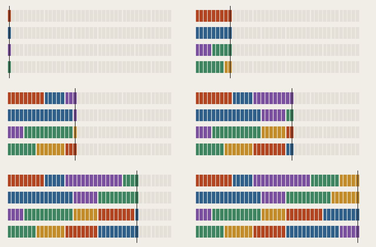
Static batching waits until every request in a batch is done before starting the next one; short replies get stuck behind long ones. Continuous batching schedules at the granularity of individual decode steps, so the batch is constantly refilled.

Quantization

If decode speed is limited by how many bytes we read, the obvious move is to read fewer bytes. Quantization stores weights (and sometimes activations or the KV cache) in lower precision.

Speculative decoding

A small “draft” model guesses the next few tokens cheaply; the big model checks all of the guesses in a single parallel pass and keeps the longest prefix it agrees with. When the draft is right, you get several tokens for the price of one big-model step. When it is wrong, you lose very little.

Self-hosted clips use the same syntax — point it at a video file in assets/video/:

![Short description](assets/video/demo.mp4 "Your caption")

Further reading

1. Attention Is All You Need Vaswani et al., 2017
2. Efficient Memory Management for LLM Serving with PagedAttention Kwon et al., 2023
3. Fast Inference from Transformers via Speculative Decoding Leviathan et al., 2022
4. FlashAttention Dao et al., 2022